

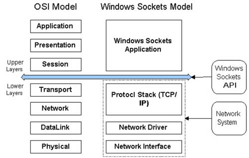
The OSI (Open System Interconnection) Model breaks the various aspects of a computer network into seven distinct layers. Each successive layer envelops the layer beneath it, hiding its details from the levels above.
The OSI Model isn't itself a networking standard in the same sense that Ethernet and TCP/IP are. Rather, the OSI Model is a framework into which the various networking standards can fit. The OSI Model specifies what aspects of a network's operation can be addressed by various network standards. So, in a sense, the OSI Model is sort of a standard's standard.
The first three layers are sometimes called the lower layers. They deal with the mechanics of how information is sent from one computer to another over a network. Layers 4–7 are sometimes called the upper layers. They deal with how applications relate to the network through application programming interfaces.
Layer 1: The Physical Layer
The bottom layer of the OSI Model is the Physical Layer. It addresses the physical characteristics of the network, such as the types of cables used to connect devices, the types of connectors used, how long the cables can be, and so on. For example, the Ethernet standard for 100BaseT cable specifies the electrical characteristics of the twisted-pair cables, the size and shape of the connectors, the maximum length of the cables, and so on.
Another aspect of the Physical Layer is that it specifies the electrical characteristics of the signals used to transmit data over cables from one network node to another. The Physical Layer doesn't define any particular meaning for those signals other than the basic binary values 0 and 1. The higher levels of the OSI model must assign meanings to the bits transmitted at the Physical Layer.
One type of Physical Layer device commonly used in networks is a repeater. A repeater is used to regenerate signals when you need to exceed the cable length allowed by the Physical Layer standard or when you need to redistribute a signal from one cable onto two or more cables.
An old-style 10BaseT hub is also a Physical Layer device. Technically, a hub is a multi-port repeater because its purpose is to regenerate every signal received on any port on all the hub's other ports. Repeaters and hubs don't examine the contents of the signals that they regenerate. If they did, they'd be working at the Data Link Layer, not at the Physical Layer.
Layer 2: The Data Link Layer
The Data Link Layer is the lowest layer at which meaning is assigned to the bits that are transmitted over the network. Data-link protocols address things, such as the size of each packet of data to be sent, a means of addressing each packet so that it's delivered to the intended recipient, and a way to ensure that two or more nodes don't try to transmit data on the network at the same time.
The Data Link Layer also provides basic error detection and correction to ensure that the data sent is the same as the data received. If an uncorrectable error occurs, the data-link standard must specify how the node is to be informed of the error so it can retransmit the data.
At the Data Link Layer, each device on the network has an address known as the Media Access Control address, or MAC address. This is the actual hardware address, assigned to the device at the factory.
You can see the MAC address for a computer's network adapter by opening a command window and running the ipconfig /all command.
Layer 3: The Network Layer
The Network Layer handles the task of routing network messages from one computer to another. The two most popular Layer-3 protocols are IP (which is usually paired with TCP) and IPX (normally paired with SPX for use with Novell and Windows networks).
One important function of the Network Layer is logical addressing. Every network device has a physical address called a MAC address, which is assigned to the device at the factory. When you buy a network interface card to install in a computer, the MAC address of that card can't be changed. But what if you want to use some other addressing scheme to refer to the computers and other devices on your network? This is where the concept of logical addressing comes in; a logical address gives a network device a place where it can be accessed on the network — using an address that you assign.
Logical addresses are created and used by Network Layer protocols, such as IP or IPX. The Network Layer protocol translates logical addresses to MAC addresses. For example, if you use IP as the Network Layer protocol, devices on the network are assigned IP addresses, such as 207.120.67.30. Because the IP protocol must use a Data Link Layer protocol to actually send packets to devices, IP must know how to translate the IP address of a device into the correct MAC address for the device. You can use the ipconfig command to see the IP address of your computer.
Another important function of the Network layer is routing — finding an appropriate path through the network. Routing comes into play when a computer on one network needs to send a packet to a computer on another network. In this case, a Network Layer device called a router forwards the packet to the destination network. An important feature of routers is that they can be used to connect networks that use different Layer-2 protocols. For example, a router can be used to connect a local-area network that uses Ethernet to a wide-area network that runs on a different set of low-level protocols, such as T1.
Layer 4: The Transport Layer
The Transport Layer is the basic layer at which one network computer communicates with another network computer. The Transport Layer is where you'll find one of the most popular networking protocols: TCP. The main purpose of the Transport Layer is to ensure that packets move over the network reliably and without errors. The Transport Layer does this by establishing connections between network devices, acknowledging the receipt of packets, and resending packets that aren't received or are corrupted when they arrive.
In many cases, the Transport Layer protocol divides large messages into smaller packets that can be sent over the network efficiently. The Transport Layer protocol reassembles the message on the receiving end, making sure that all packets contained in a single transmission are received and no data is lost.
Layer 5: The Session Layer
The Session Layer establishes sessions (instances of communication and data exchange) between network nodes. A session must be established before data can be transmitted over the network. The Session Layer makes sure that these sessions are properly established and maintained.
Layer 6: The Presentation Layer
The Presentation Layer is responsible for converting the data sent over the network from one type of representation to another. For example, the Presentation Layer can apply sophisticated compression techniques so fewer bytes of data are required to represent the information when it's sent over the network. At the other end of the transmission, the Transport Layer then uncompresses the data.
The Presentation Layer also can scramble the data before it's transmitted and then unscramble it at the other end, using a sophisticated encryption technique.
Layer 7: The Application Layer
The highest layer of the OSI model, the Application Layer, deals with the techniques that application programs use to communicate with the network. The name of this layer is a little confusing because application programs (such as Excel or Word) aren't actually part of the layer. Rather, the Application Layer represents the level at which application programs interact with the network, using programming interfaces to request network services. One of the most commonly used application layer protocols is HTTP, which stands for HyperText Transfer Protocol. HTTP is the basis of the World Wide Web.
Unix standards:
The 1973 rewrite of Unix in C made it unprecedentedly easy to port and modify. As a result, the ancestral Unix diverged into a family of operating systems early on. Unix standards originally developed to reconcile the APIs of the different branches of the family tree.
The Unix standards that evolved after 1985 were quite successful at this — so much so that they serve as valuable documentation of the API of modern Unix implementations. In fact, real-world Unixes follow published standards so closely that developers can (and frequently do) lean more on documents like the POSIX specification than on the official manual pages for the Unix variant they happen to be using.
In fact, on the newer open-source Unixes (such as Linux), it is common for operating-system features to have been engineered using published standards as the specification. We'll return to this point when we examine the RFC standards process later in this chapter.
Standards and the Unix Wars
The original motivation for the development of Unix standards was the split between the AT&T and Berkeley lines of development that we examined in
The 4.x BSD Unixes were descended from the 1979 Version 7. After the release of 4.1BSD in 1980 the BSD line quickly developed a reputation as the cutting edge of Unix. Important additions included the vi visual editor, job control facilities for managing multiple foreground and background tasks from a single console, and improvements in signals By far the most important addition was to be TCP/IP networking, but though Berkeley got the contract to do it in 1980, TCP/IP was not to ship in an external release for three years.
But another version, 1981's System III, became the basis of AT&T's later development. System III reworked the Version 7 terminals interface into a cleaner and more elegant form that was completely incompatible with the Berkeley enhancements. It retained the older (non-resetting) semantics of signals (again, see Chapter 7 for discussion of this point). The January 1983 release of System V Release 1 incorporated some BSD utilities (such as vi(1)).
The first attempt to bridge the gap came in February 1983 from UniForum, an influential Unix user group. Their Uniforum 1983 Draft Standard (UDS 83) described a “core Unix System” consisting of a subset of the System III kernel and libraries plus a file-locking primitive. AT&T declared support for UDS 83, but the standard was an inadequate subset of evolving practice based on 4.1BSD. The problem was exacerbated by the July 1983 release of 4.2BSD, which added many new features (including TCP/IP networking) and introduced some subtle incompatibilities with the ancestral Version 7.
The 1984 divestiture of the Bell operating companies and the beginnings of the Unix wars significantly complicated matters. Sun Microsystems was leading the workstation industry in a BSD direction; AT&T was trying to get into the computer business and use control of Unix as a strategic weapon even as it continued to license the operating system to competitors like Sun. All the vendors were making business decisions to differentiate their versions of Unix for competitive advantage.
During the Unix wars, technical standardization became something that cooperating technical people pushed for and most product managers accepted grudgingly or actively resisted. The one large and important exception was AT&T, which declared its intention to cooperate with user groups in setting standards when it announced System V Release 2 (SVr2) in January 1984. The second revision of the UniForum Draft Standard, in 1984, both tracked and influenced the API of SVr2. Later Unix standards also tended to track System V except in areas where BSD facilities were clearly functionally superior (thus, for example, modern Unix standards describe the System V terminal controls rather than the BSD interface to the same facilities).
In 1985, AT&T released the System V Interface Definition (SVID). SVID provided a more formal description of the SVr2 API, incorporating UDS 84. Later revisions SVID2 and SVID3 tracked the interfaces of System V releases 3 and 4. SVID became the basis for the POSIX standards, which ultimately tipped most of the Berkeley/AT&T disputes over system and C library calls in AT&T's favor.
But this would not become obvious for a few years yet; meanwhile, the Unix wars raged on. For example, 1985 saw the release of two competing API standards for file system sharing over networks: Sun's Network File System (NFS) and AT&T's Remote File System (RFS). Sun's NFS prevailed because Sun was willing to share not merely specifications but open-source code with others.
The lesson of this success should have been all the more pointed because on purely logical grounds RFS was the superior model. It supported better file-locking semantics and better mapping among user identities on different systems, and generally made an effort to get the finer details of Unix file system semantics precisely right, unlike NFS. The lesson was ignored, however, even when it was repeated in 1987 by the open-source X windowing system's victory over Sun's proprietary Networked Window System (NeWS).
After 1985 the main thrust of Unix standardization passed to the Institute of Electrical and Electronic Engineers (IEEE). The IEEE's 1003 committee developed a series of standards generally known as POSIX.[144] These went beyond describing merely systems calls and C library facilities; they specified detailed semantics of a shell and a minimum command set, and also detailed bindings for various non-C programming languages. The first release in 1990 was followed by a second edition in 1996. The International Standards Organization adopted them as ISO/IEC 9945.
Key POSIX standards include the following: Library procedures, described the C system call API, much like Version 7 except for signals and the terminal-control interface.
- 1003.2 (released 1992)
Standard shell and utilities. Shell semantics strongly resemble those of the System V Bourne shell.
- 1003.4 (released 1993)
Real-time Unix. Binary semaphores, process memory locking, memory-mapped files, shared memory, priority scheduling, real-time signals, clocks and timers, IPC message passing, synchronized I/O, asynchronous I/O, real-time files.
In the 1996 Second Edition, 1003.4 was split into 1003.1b (real-time) and 1003.1c (threads).
Despite being underspecified in a couple of key areas such as signal-handling semantics and omitting BSD sockets, the original POSIX standards became the basis of all later Unix standardization work. They are still cited as an authority, albeit indirectly through references like POSIX Programmer's Guide [Lewine]. The de facto Unix API standard is still “POSIX plus sockets”, with later standards mainly adding features and specifying conformance in unusual edge cases more closely.
The next player on the scene was X/Open (later renamed the Open Group), a consortium of Unix vendors formed in 1984. Their X/Open Portability Guides (XPGs) initially developed in parallel with the POSIX drafts, then after 1990 the XPGs incorporated and extended POSIX. Unlike POSIX, which attempted to capture a safe subset of all Unixes, the XPGs were oriented more toward common practice at the leading edge; even XPG1 in 1985, spanning SVr2 and 4.2BSD, included sockets.
XPG2 in 1987 added a terminal-handling API that was essentially System V curses(3). XPG3 in 1990 merged in the X11 API. XPG4 in 1992 mandated full compliance with the 1989 ANSI C standard. XPG2, 3, and 4 were heavily concerned with support of internationalization and described an elaborate API for handling code sets and message catalogs.
In reading about Unix standards you might come across references to “Spec 1170” (from 1993), “Unix 95” (from 1995) and “Unix 98” (from 1998). These were certification marks based on the X/Open standards; they are now of historical interest only. But the work done on XPG4 turned into Spec 1170, which turned into the first version of the Single Unix Specification (SUS).
In 1993 seventy-five systems and software vendors including every major Unix company put a final end to the Unix wars when they declared backing for X/Open to develop a common definition of Unix. As part of the arrangement, X/Open acquired the rights to the Unix trademark. The merged standard became Single Unix Standard version 1. It was followed in 1997 by a version 2. In 1999 X/Open absorbed the POSIX activity.
In 2001, X/Open (now The Open Group) issued the Single Unix Standard version 3. All the threads of Unix API standardization were finally gathered into one bundle. This reflected facts on the ground; the different varieties of Unix had re-converged on a common API. And, at least among old-timers who remembered the turbulence of the 1980s, there was much rejoicing.
The Ghost at the Victory Banquet
There was, unfortunately, an awkward detail — the old-school Unix vendors who had backed the effort were under severe pressure from the new school of open-source Unixes, and were in some cases in the process of abandoning (in favor of Linux) the proprietary Unixes for which they had gone to so much effort to secure conformance.
The conformance testing needed to verify Single Unix Specification conformance is an expensive proposition. It would need to be done on a per-distribution basis, but is well out of the reach of most distributors of open-source operating systems. In any case, Linux changes so fast that any given release of a distribution would probably be obsolete by the time it could get certified.
Standards like the Single Unix Specification have not entirely lost their relevance. They're still valuable guides for Unix implementers. But how The Open Group and other institutions of the old-school Unix standardization process will adapt to the rapid tempo of open-source releases (and to the low- or zero-budget operation of open-source development groups!) remains to be seen.
Unix Standards in the Open-Source World
In the mid-1990s, the open-source community began standardization efforts of its own. These efforts built on the source-code-level compatibility secured by POSIX and its descendants. Linux, in particular, had been written from scratch in a way that depended on the availability of Unix API standards like POSIX
In 1998 Oracle ported its market-leading database product to Linux, in a move that was rightly seen as a major breakthrough in Linux's mainstream acceptance. The engineer in charge of the port provided a definitive demonstration that API standards had done their job when he was asked by a reporter what technical challenges Oracle had had to surmount. The engineer's reply was “We typed ‘make’.”
The problem for the new-school Unixes, therefore, was not API compatibility at the source-code level. Everybody took for granted the ability to move source code between different Linux, BSD, and proprietary-Unix distributions without more than a trivial amount of porting labor. The new problem was not source compatibility but binary compatibility. For the ground under Unix had shifted in a subtle way as a consequence of the triumph of commodity PC hardware.
In the old days, each Unix had run on what was effectively its own hardware platform. There was enough variety in processor instruction sets and machine architectures that applications had to be ported at source level to move at all. On the other hand, there were a relatively few major Unix releases, each with relatively long service lifetimes. Application vendors like Oracle could afford the cost of building and shipping separate binary distributions for each of three or four hardware/software combinations, because they could amortize the low cost of source-code porting over large customer populations and a long enough product life cycle.
But then the minicomputer and workstation vendors were swamped by inexpensive 386-based supermicros, and open-source Unixes changed the rules. Vendors found they no longer had a stable platform to ship their binaries to.
The superficial problem, at first, was the large number of Unix distributors — but as the Linux distribution market consolidated, it became clear that the real issue was the rate of change over time. APIs were stable, but the expected locations of system administrative files, utility programs, and things like the prefix of the paths to user mailbox names and system log files kept changing.
The first standards effort to develop within the new-school Linux and BSD community itself (beginning in 1993) was the Filesystem Hierarchy Standard (FHS). This was incorporated into the Linux Standards Base (LSB), which also standardized an expected set of service libraries and helper applications. Both standards became activities of the Free Standards Group, which by 2001 developed a role similar to X/Open's position amidst the old-school Unix vendors.
TCP Connection Establishment Process: The "Three-Way Handshake"
We have discussed in earlier topics in this section the connection orientation of TCP and its operation. Before TCP can be employed for any actually useful purpose—that is, sending data—a connection must be set up between the two devices that wish to communicate. This process, usually called connection establishment, involves an exchange of messages that transitions both devices from their initial connection state (CLOSED) to the normal operating state (ESTABLISHED).
Connection Establishment Functions
The connection establishment process actually accomplishes several things as it creates a connection suitable for data exchange:
- Contact and Communication: The client and server make contact with each other and establish communication by sending each other messages. The server usually doesn’t even know what client it will be talking to before this point, so it discovers this during connection establishment.
- Sequence Number Synchronization: Each device lets the other know what initial sequence number it wants to use for its first transmission.
- Parameter Exchange: Certain parameters that control the operation of the TCP connection are exchanged by the two devices.
Buffer sizes and limitation:
Certain limits affect the size of IP datagrams. We first describe these limits and then tie them all together with regard to how they affect the data an application can transmit.
- The maximum size of an IPv4 datagram is 65,535 bytes, including the IPv4 header. This is because of the 16-bit total length field in Figure A.1.
- The maximum size of an IPv6 datagram is 65,575 bytes, including the 40-byte IPv6 header. This is because of the 16-bit payload length field in Figure A.2. Notice that the IPv6 payload length field does not include the size of the IPv6 header, while the IPv4 total length field does include the header size.
IPv6 has a jumbo payload option, which extends the payload length field to 32 bits, but this option is supported only on datalinks with a maximum transmission unit (MTU) that exceeds 65,535. (This is intended for host-to-host interconnects, such as HIPPI, which often have no inherent MTU.)
- Many networks have an MTU which can be dictated by the hardware. For example, the Ethernet MTU is 1,500 bytes. Other datalinks, such as point-to-point links using the Point-to-Point Protocol (PPP), have a configurable MTU. Older SLIP links often used an MTU of 1,006 or 296 bytes.
The minimum link MTU for IPv4 is 68 bytes. This permits a maximum-sized IPv4 header (20 bytes of fixed header, 30 bytes of options) and minimum- sized fragment (the fragment offset is in units of 8 bytes). The minimum link MTU for IPv6 is 1,280 bytes. IPv6 can run over links with a smaller MTU, but requires link-specific fragmentation and reassembly to make the link appear to have an MTU of at least 1,280 bytes (RFC 2460 [Deering and Hinden 1998]).
- The smallest MTU in the path between two hosts is called the path MTU . Today, the Ethernet MTU of 1,500 bytes is often the path MTU. The path MTU need not be the same in both directions between any two hosts because routing in the Internet is often asymmetric [Paxson 1996]. That is, the route from A to B can differ from the route from B to A.
- When an IP datagram is to be sent out an interface, if the size of the datagram exceeds the link MTU, fragmentation is performed by both IPv4 and IPv6. The fragments are not normally reassembled until they reach the final destination. IPv4 hosts perform fragmentation on datagrams that they generate and IPv4 routers perform fragmentation on datagrams that they forward. But with IPv6, only hosts perform fragmentation on datagrams that they generate; IPv6 routers do not fragment datagrams that they are forwarding.
- We must be careful with our terminology. A box labeled as an IPv6 router may indeed perform fragmentation, but only on datagrams that the router itself generates, never on datagrams that it is forwarding. When this box generates IPv6 datagrams, it is really acting as a host. For example, most routers support the Telnet protocol and this is used for router configuration by administrators. The IP datagrams generated by the router's Telnet server are generated by the router, not forwarded by the router.
- You may notice that fields exist in the IPv4 header (Figure A.1) to handle IPv4 fragmentation, but there are no fields in the IPv6 header (Figure A.2) for fragmentation. Since fragmentation is the exception, rather than the rule, IPv6 contains an option header with the fragmentation information.
- Certain firewalls, which usually act as routers, may reassemble fragmented packets to allow inspection of the entire packet contents. This allows the prevention of certain attacks at the cost of additional complexity in the firewall device. It also requires the firewall device to be part of the only path to the network, reducing the opportunities for redundancy.
- If the "don't fragment" (DF) bit is set in the IPv4 header (Figure A.1), it specifies that this datagram must not be fragmented, either by the sending host or by any router. A router that receives an IPv4 datagram with the DF bit set whose size exceeds the outgoing link's MTU generates an ICMPv4 "destination unreachable, fragmentation needed but DF bit set" error message (Figure A.15).
- Since IPv6 routers do not perform fragmentation, there is an implied DF bit with every IPv6 datagram. When an IPv6 router receives a datagram whose size exceeds the outgoing link's MTU, it generates an ICMPv6 "packet too big" error message (Figure A.16).
- The IPv4 DF bit and its implied IPv6 counterpart can be used for path MTU discovery (RFC 1191 [Mogul and Deering 1990] for IPv4 and RFC 1981 [McCann, Deering, and Mogul 1996] for IPv6). For example, if TCP uses this technique with IPv4, then it sends all its datagrams with the DF bit set. If some intermediate router returns an ICMP "destination unreachable, fragmentation needed but DF bit set" error, TCP decreases the amount of data it sends per datagram and retransmits. Path MTU discovery is optional with IPv4, but IPv6 implementations all either support path MTU discovery or always send using the minimum MTU.
- Path MTU discovery is problematic in the Internet today; many firewalls drop all ICMP messages, including the fragmentation required message, meaning that TCP never gets the signal that it needs to decrease the amount of data it is sending. As of this writing, an effort is beginning in the IETF to define another method for path MTU discovery that does not rely on ICMP errors.
- IPv4 and IPv6 define a minimum reassembly buffer size , the minimum datagram size that we are guaranteed any implementation must support. For IPv4, this is 576 bytes. IPv6 raises this to 1,500 bytes. With IPv4, for example, we have no idea whether a given destination can accept a 577-byte datagram or not. Therefore, many IPv4 applications that use UDP (e.g., DNS, RIP, TFTP, BOOTP, SNMP) prevent applications from generating IP datagrams that exceed this size.
- TCP has a maximum segment size (MSS) that announces to the peer TCP the maximum amount of TCP data that the peer can send per segment. We saw the MSS option on the SYN segments in Figure 2.5. The goal of the MSS is to tell the peer the actual value of the reassembly buffer size and to try to avoid fragmentation. The MSS is often set to the interface MTU minus the fixed sizes of the IP and TCP headers. On an Ethernet using IPv4, this would be 1,460, and on an Ethernet using IPv6, this would be 1,440. (The TCP header is 20 bytes for both, but the IPv4 header is 20 bytes and the IPv6 header is 40 bytes.)
- The MSS value in the TCP MSS option is a 16-bit field, limiting the value to 65,535. This is fine for IPv4, since the maximum amount of TCP data in an IPv4 datagram is 65,495 (65,535 minus the 20-byte IPv4 header and minus the 20-byte TCP header). But with the IPv6 jumbo payload option, a different technique is used (RFC 2675 [Borman, Deering, and Hinden 1999]). First, the maximum amount of TCP data in an IPv6 datagram without the jumbo payload option is 65,515 (65,535 minus the 20-byte TCP header). Therefore, the MSS value of 65,535 is considered a special case that designates "infinity." This value is used only if the jumbo payload option is being used, which requires an MTU that exceeds 65,535. If TCP is using the jumbo payload option and receives an MSS announcement of 65,535 from the peer, the limit on the datagram sizes that it sends is just the interface MTU. If this turns out to be too large (i.e., there is a link in the path with a smaller MTU), then path MTU discovery will determine the smaller value.
- SCTP keeps a fragmentation point based on the smallest path MTU found to all the peer's addresses. This smallest MTU size is used to split large user messages into smaller pieces that can be sent in one IP datagram. The SCTP_MAXSEG socket option can influence this value, allowing the user to request a smaller fragmentation point.
TCP Output
Given all these terms and definitions, Figure 2.15 shows what happens when an application writes data to a TCP socket.
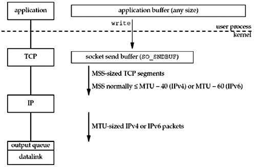
Figure 2.15. Steps and buffers involved when an application writes to a TCP socket
Every TCP socket has a send buffer and we can change the size of this buffer with the SO_SNDBUF socket option (Section 7.5). When an application calls write , the kernel copies all the data from the application buffer into the socket send buffer. If there is insufficient room in the socket buffer for all the application's data (either the application buffer is larger than the socket send buffer, or there is already data in the socket send buffer), the process is put to sleep. This assumes the normal default of a blocking socket. (We will talk about nonblocking sockets in Chapter 16.) The kernel will not return from the write until the final byte in the application buffer has been copied into the socket send buffer. Therefore, the successful return from a write to a TCP socket only tells us that we can reuse our application buffer. It does not tell us that either the peer TCP has received the data or that the peer application has received the data. (We will talk about this more with the SO_LINGER socket option in Section 7.5.)
TCP takes the data in the socket send buffer and sends it to the peer TCP based on all the rules of TCP data transmission (Chapter 19 and 20 of TCPv1). The peer TCP must acknowledge the data, and as the ACKs arrive from the peer, only then can our TCP discard the acknowledged data from the socket send buffer. TCP must keep a copy of our data until it is acknowledged by the peer.
TCP sends the data to IP in MSS-sized or smaller chunks , prepending its TCP header to each segment, where the MSS is the value announced by the peer, or 536 if the peer did not send an MSS option. IP prepends its header, searches the routing table for the destination IP address (the matching routing table entry specifies the outgoing interface), and passes the datagram to the appropriate datalink. IP might perform fragmentation before passing the datagram to the datalink, but as we said earlier, one goal of the MSS option is to try to avoid fragmentation and newer implementations also use path MTU discovery. Each datalink has an output queue, and if this queue is full, the packet is discarded and an error is returned up the protocol stack: from the datalink to IP and then from IP to TCP. TCP will note this error and try sending the segment later. The application is not told of this transient condition.
UDP Output
Figure 2.16 shows what happens when an application writes data to a UDP socket.
Figure 2.16. Steps and buffers involved when an application writes to a UDP socket.
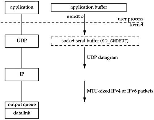
UDP simply prepends its 8-byte header and passes the datagram to IP. IPv4 or IPv6 prepends its header, determines the outgoing interface by performing the routing function, and then either adds the datagram to the datalink output queue (if it fits within the MTU) or fragments the datagram and adds each fragment to the datalink output queue. If a UDP application sends large datagrams (say 2,000-byte datagrams), there is a much higher probability of fragmentation than with TCP, because TCP breaks the application data into MSS-sized chunks, something that has no counterpart in UDP.
The successful return from a write to a UDP socket tells us that either the datagram or all fragments of the datagram have been added to the datalink output queue. If there is no room on the queue for the datagram or one of its fragments, ENOBUFS is often returned to the application.
Unfortunately, some implementations do not return this error, giving the application no indication that the datagram was discarded without even being transmitted.
SCTP Output
Figure 2.17 shows what happens when an application writes data to an SCTP socket.
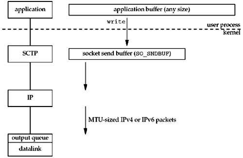
SCTP, since it is a reliable protocol like TCP, has a send buffer. As with TCP, an application can change the size of this buffer with the SO_SNDBUF socket option (Section 7.5). When the application calls write , the kernel copies all the data from the application buffer into the socket send buffer. If there is insufficient room in the socket buffer for all of the application's data (either the application buffer is larger than the socket send buffer, or there is already data in the socket send buffer), the process is put to sleep. This sleeping assumes the normal default of a blocking socket. (We will talk about nonblocking sockets in Chapter 16.) The kernel will not return from the write until the final byte in the application buffer has been copied into the socket send buffer. Therefore, the successful return from a write to an SCTP socket only tells the sender that it can reuse the application buffer. It does not tell us that either the peer SCTP has received the data, or that the peer application has
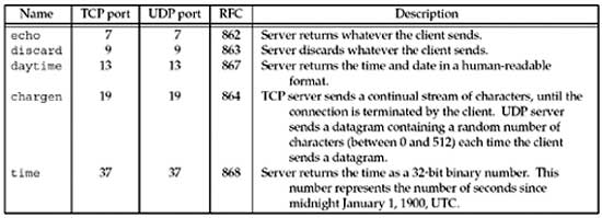
Standard Internet Services
Figure 2.18 lists several standard services that are provided by most implementations of TCP/IP. Notice that all are provided using both TCP and UDP and the port number is the same for both protocols.
| aix % telnet freebsd daytime | |
| Trying 12.106.32.254... | output by Telnet client |
| Connected to freebsd.unpbook.com. | output by Telnet client |
| Escape character is '^]'. | output by Telnet client |
| Mon Jul 28 11:56:22 2003 | output by daytime server |
| Connection closed by foreign host. | output by Telnet client (server closes connection) |
| aix % telnet freebsd echo | |
| Trying 12.106.32.254... | output by Telnet client |
| Connected to freebsd.unpbook.com. | output by Telnet client |
| Escape character is '^]'. | output by Telnet client |
| hello, world | we type this |
| hello , world | and it is echoed back by the server |
| ^] | we type control and right bracket to talk to Telnet client |
| telnet> quit | and tell client we are done |
| Connection closed. | client closes the connection this time |
In these two examples, we type the name of the host and the name of the service ( daytime and echo ). These service names are mapped into the port numbers shown in Figure 2.18 by the /etc/services file, as we will describe in Section 11.5.
Notice that when we connect to the daytime server, the server performs the active close, while with the echo server, the client performs the active close. Recall from Figure 2.4 that the end performing the active close is the end that goes through the TIME_WAIT state.
These "simple services" are often disabled by default on modern systems due to denial-of-service and other resource utilization attacks against them.
Protocol Usage by Common Internet Applications
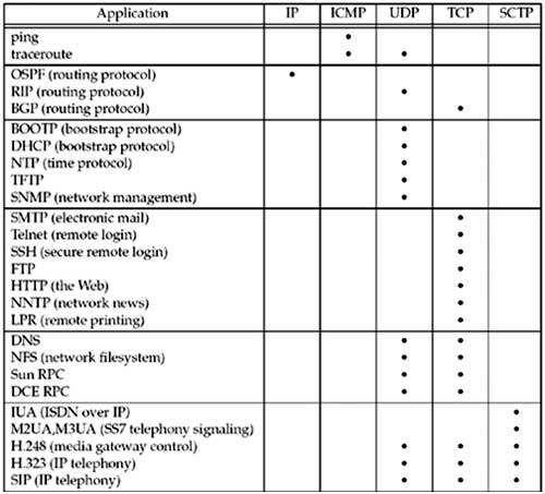
The three popular routing protocols demonstrate the variety of transport protocols used by routing protocols. OSPF uses IP directly, employing a raw socket, while RIP uses UDP and BGP uses TCP.
The next five are UDP-based applications, followed by seven TCP applications and four that use both UDP and TCP. The final five are IP telephony applications that use SCTP exclusively or optionally UDP, TCP, or SCTP.