


Causes: Bursty nature of tra?c is the root cause ? when a part of the network no longer can cope up a sudden increase of tra?c, congestion builds upon. Other factors, such as lack of bandwidth, ill-configuration and slow routers can also bring up congestion.
Di?erences between Congestion Control and Flow Control:
Congestion control try to make sure that subnet can carry offered traffic, a global issue involving all the hosts and routers. It can be open-loop based or involving feedback
Flow control is related to point-to-point tra?c between given sender and receiver, it always involves direct feedback from receiver to sender
TCP Congestion Control Algorithms:
Congestion control algorithms exist for different types of TCPs. For standard TCP, following are the algorithms designed:
Standard TCP:
The algorithms used are:
- Slow Start
- Congestion Avoidance
- Fast Retransmit
- Fast Recovery.
A TCP connection is always using one of these four algorithms throughout the life of the connection.
Slow Start:
After a TCP connection is established, initial congestion algorithm used is the Slow Start algorithm. During the slow start, congestion window is incremented by one segment for every new ACK received. The connection remains in slow start until one of three events occurs.
WHAT IS SLOW-START-THRESHOLD (ssthresh)?
It is the value given by the receiver to the sender. By refereeing this value, sender maintains the sending
The first event is when congestion window reaches the slow start threshold. The connection then uses congestion avoidance algorithm, after the congestion window is greater than, or equal to, the slow start threshold. The slow start threshold, ssthresh, is a variable used to determine when the connection should change from the slow start algorithm to congestion avoidance algorithm. The initial value of ssthresh is set to an arbitrarily high value; this value is not usually reached during initial slow start after a new connection is established.
The second event is receiving the duplicate ACKs for same data. Upon receiving three duplicate ACKs, the connection uses fast retransmit algorithm.
The third event that can occur during slow start is a timeout. If a timeout occurs, congestion avoidance algorithm is used to adjust congestion window and slow start threshold.
Congestion Avoidance:
The congestion avoidance algorithm consists of two parts,
- Additive Increment (AI)
- Multiplicative Decrement (MD)
It referred to as AIMD. When congestion avoidance occurs, additive increment is used to adjust congestion window after receiving new ACKs. Multiplicative decrement is used to adjust congestion window after a congestion event occurs.
Additive Increment:
After receiving an ACK for new data, congestion window is increment by (MSS)2/Cwnd, where, MSS is maximum segment size, this formula is known as additive increment. The goal of additive increment is to open congestion window by a maximum of one MSS per RTT. Additive increment can be described by using the following equation:
Cwnd= Cwnd+ a*MSS2/Cwnd, where the value of a is a constant, a = 1.
The maximum segment size (MSS) is a parameter of the TCP protocol that specifies the largest amount of data, specified in octets, that a computer or communications device can receive in a single TCPsegment. It does not count the TCP header or the IP header.
Multiplicative Decrement:
Multiplicative decrement occurs after a congestion event, such as a lost packet or a timeout. After a congestion event occurs, the slow start threshold is set to half current congestion window. This update to slow start threshold follows equation:
ssthresh = (1-b)*FlightSize
FlightSize is equal to amount of data that has been sent but not yet ACKed and b is a constant, b = 0.5. The congestion window is adjusted accordingly. After a timeout occurs, congestion window is set to one MSS and slow start algorithm is reuse.
The fast retransmit and fast recovery algorithms covers congestion events due to lost packets.
Fast Retransmit:
The fast retransmit algorithm was designed for quick recovery from a lost packet before a timeout occurs. When sending data, fast retransmit algorithm is used after receiving three duplicate ACKs for same segment. After receiving duplicate ACKs, sender immediately resend the lost packets, to avoid a timeout, and then use the fast recovery algorithm.
Fast Recovery:
Fast Recovery algorithm is used to avoid setting the congestion window equal to one MSS segment after a drop packet occurs. After a drop occurs, multiplicative decrement portion of congestion avoidance is used to update the slow start threshold. Next, the congestion window is set to a new value of ssthresh. After the window size is decremented, additive increment is used to reopen congestion window.
Figure shows the example of outstanding data for a TCP connection and illustrates the performance of congestion control. The connection starts using slow start algorithm until the channel is filled and then switches congestion avoidance.
Fig.: Standard TCP Congestion Control.
In this example, a single drop occurs around three seconds. Fast Retransmit and Recovery algorithms are used to resend lost segment and then cut congestion window in half. Additive increment is used after the drop to reopen the congestion window.
Concatenated Virtual Circuits
A virtual circuit is a circuit or path between points in a network that appears to be a discrete physical path, but is actually a managed pool of circuit resources from which specific circuits are allocated as needed to meet traffic requirements.
A permanent virtual circuit (PVC) is a virtual circuit that is permanently available to the user just as though it were a dedicated or leased line continuously reserved for that user. A switched virtual circuit (SVC) is a virtual circuit in which a connection session is set up for a user only for the duration of a connection. PVCs are an important feature of frame relay networks and SVCs are proposed for later inclusion.
Two styles of internetworking are possible
1.Concatenated Virtual Circuit Model:
This is similar to a connection-oriented approach. The subnet sees that the destination is remote and builds a Virtual circuit to the router nearest the destination network. Then it constructs a virtual circuit from that router to an external gateway. This gateway records the existence of the virtual circuit in its tables and proceeds in the next subnet. This process continues until the destination host has been reached. Once data packets begins flowing along the path, each gateway relays incoming packets, converting between packet formats and virtual circuit numbers as needed. Clearly all data packets must traverse the same sequence of gateways. Consequently packets in a flow are never reordered by the network.
- CVC is End-to-End connection that consists of several consecutive point to point links between
- Source host and subnet
- Subnet ad multi protocol router (“full gateway”)
- Subnet and subnet connected by shared “half gateway”
- Subnet and destined host
- Features:
- The data routes are identified by VC numbers
- During the session data packets transverse the same sequence of GWs and arrive in order
- The routers are supported by VC tables containing
- The ID number of actual VC
- Next destination for each VC
- The number of the next concatenated VCs
- Buffers can be reserved in advance
- sequencing can be guaranteed
- short headers can be used
- Troubles caused by delayed duplicate packets can be avoided.
- Table space required in the routers for each open connection.
- No alternate routing to avoid congested areas.
- Vulnerability to router failures along the path
This is similar to a connection-less approach. In this model the only service the network layer offers to the transport layer is the ability to inject datagrams into the subnet and hope for the best. There is no notion of a Virtual Circuit at all in the network layer, let alone a concatenation of them. It does not require all packets belonging to one connection to traverse the same sequence of gateways. Routing decision is made separately for each packet, possibly depending on the traffic at the moment the packet is sent. It can use multiple routes and thus achieve a higher bandwidth than the concatenated virtual circuit model. There is no guarantee that the packets arrive at the destination in order, assuming that they arrive at all.
- Robustness in the face of router failures.
- Can be used over subnets that do not use Virtual circuits inside
- More potential for congestion.
- Longer headers are needed.
- No sequencing.
Datagrams are constructed and sent in the usual way. Routing decisions are made on a packet by packet basis so that we cannot even guarantee that all the packets in a message will be sent over the same set of networks. Since each of the networks can have different properties, the processing that the packets receive will be different depending on the route they took.
Since each network will have its own network layer protocol we cannot simply transfer network layer packets across the routers. One possibility is to try and convert from one protocol to another, but this is not very successful for much the same set of reasons that converting between the different frame types of the 802 Ethernets was difficult.
A major issue in transferring from one network to another is that of addressing. In general different networks use different addressing schemes. One possibility would be to assign every host an address for every sort of network but apart from being inefficient (lots of addresses would never be used) it would also require a huge translation table to be kept.
IP (Internet Protocol) attempts to do is to define a universal packet which can be carried across all networks. Of course others have also had this idea so there are several ‘universal’ schemes and these have to be dealt with as well.
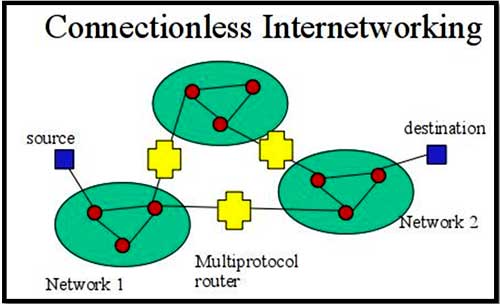
Series of datagram networks are joined together at the network layer by Multiprotocol Routers to make larger datagram network.
Connectionless verses Connection oriented Internets
Connection-oriented internetworks have much the same problems as connection oriented subnets. But they also have the same disadvantages:
- Connection-oriented internetworks are difficult, if not impossible to run across datagram subnets.
- Connectionless internetworks have much the same characteristics as connectionless subnets.
- Connectionless internets can run across both datagram and virtual circuit subnets.
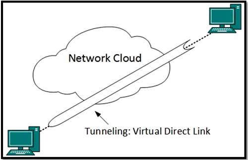
Tunneling
It is also called as Post-Forwarding. In tunneling, the data are broken into smaller pieces called packets as they move along the tunnel for transport. As the packets move through the tunnel, they are encrypted and another process called encapsulation occurs. The private network data and the protocol information that goes with it are encapsulated in public network transmission units for sending. The units look like public data, allowing them to be transmitted across the Internet. Encapsulation allows the packets to arrive at their proper destination. At the final destination, de-capsulation and decryption occur.
There are various protocols that allow tunneling to occur, including:
- Point-to-Point Tunneling Protocol (PPTP): PPTP keeps proprietary data secure even when it is being communicated over public networks. Authorized users can access a private network called a virtual private network, which is provided by an Internet service provider. This is a private network in the “virtual” sense because it is actually being created in a tunneled environment.
- Layer Two Tunneling Protocol (L2TP): This type of tunneling protocol involves a combination of using PPTP and Layer 2 Forwarding.
Tunneling is a way for communication to be conducted over a private network but tunneled through a public network. This is particularly useful in a corporate setting and also offers security features such as encryption options.
The tunneling protocol works by using the data portion of a packet (the payload) to carry the packets that actually provide the service. Tunneling uses a layered protocol model such as those of the OSI or TCP/IP protocol suite, but usually violates the layering when using the payload to carry a service not normally provided by the network. Typically, the delivery protocol operates at an equal or higher level in the layered model than the payload protocol.
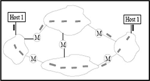
If they are two geographically separate networks, which want to communicate with each other, they may deploy a dedicated line between or they have to pass their data through intermediate networks.
Tunneling is a mechanism by which two or more same networks communicate with each other, by passing intermediate networking complexities. Tunneling is configured at both ends.
Data when enters from one end of Tunnel, it is tagged. This tagged data is then routed inside the intermediate or transit network to reach the other end of Tunnel. When data exists the Tunnel its tag is removed and delivered to the other part of the network.
Both ends feel as if they are directly connected and tagging makes data travel through transit network without any modifications.
INTERNETWORK ROUTING
The following terms are essential to your understanding of routing:
End Systems: As defined by the International Standards Organization (ISO), end systems are network devices without the ability to forward packets between portions of a network. End systems are also known as hosts.
Intermediate Systems: Network devices with the ability to forward packets between portions of a network. Bridges, switches, and routers are examples of intermediate systems.
Network: A portion of the networking infrastructure (encompassing repeaters, hubs, and bridges/Layer 2 switches that is bound by a network layer intermediate system and is associated with the same network layer address.
Router: A network layer intermediate system used to connect networks together based on a common network layer protocol.
Hardware Router: A router that performs routing as a dedicated function and has specific hardware designed and optimized for routing.
Software Router: A router that is not dedicated to performing routing but performs routing as one of multiple processes running on the router computer. The Windows 2000 Server Router Service is a software router.
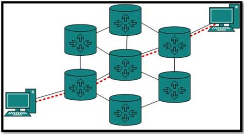
Internetwork: At least two networks connected using routers.
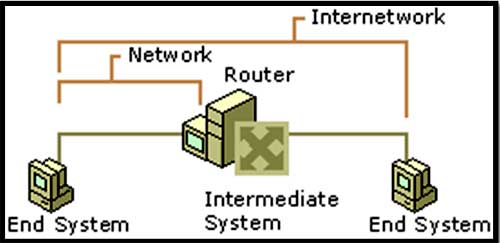
Fig.: Internetwork
Addressing in an Internetwork:
The following internetwork addressing terms are also important to your understanding of routing:
Network Address: Also known as a network ID. The number assigned to a single network in an internetwork. Network addresses are used by hosts and routers when routing a packet from a source to a destination in an internetwork.
Host Address: Also known as a host ID or a node ID. Can either be the host's physical address (the address of the network interface card) or an administratively assigned address that uniquely identifies the host on its network.
Internetwork Address: The combination of the network address and the host address; it uniquely identifies a host on an internetwork. An IP address that contains a network ID and a host ID is an internetwork address.
When a packet is sent from a source host to a destination host on an internetwork, the Network layer header of the packet contains:
- The Source Internetwork Address, which contains a source network address and source host address.
- The Destination Internetwork Address, which contains a destination network address and destination host address.
- A Hop Count, which either starts at zero and increases numerically for each router crossed to a maximum value, or starts at a maximum value and decreases numerically to zero for each router crossed. The hop count is used to prevent the packet from endlessly circulating on the internetwork.
To be more precise
In real world scenario, networks under same administration are generally scattered geographically. There may be requirement of connecting two different networks of same kind as well as of different kinds. Routing between two networks is called internetworking.
Networks can be considered different based on various parameters such as, Protocol, topology, Layer-2 network and addressing scheme.
In internetworking, routers have knowledge of each other’s address and addresses beyond them. They can be statically configured to go on different network or they can learn by using internetworking routing protocol.
Routing protocols which are used within an organization or administration are called Interior Gateway Protocols or IGP. RIP, OSPF are example of IGP. Routing between different organization or administration may have Exterior Gateway Protocol, and there is only one EGP i.e. Border Gateway Protocol.
FRAGMENTATION
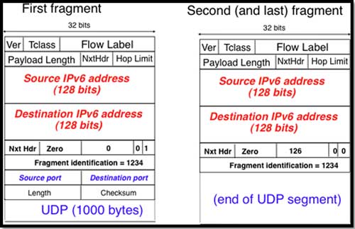
When an IP datagram travels from one host to another, it can pass through different physical networks. Each physical network has a maximum frame size. This is called the maximum transmission unit (MTU). It limits the length of a datagram that can be placed in one physical frame. IP implements a process to fragment datagrams exceeding the MTU. The process creates a set of datagrams within the maximum size.
The receiving host reassembles the original datagram. IP requires that each link support a minimum MTU of 68 octets. This is the sum of the maximum IP header length (60 octets) and the minimum possible length of data in a non-final fragment (8 octets). If any network provides a lower value than this, fragmentation and reassembly must be implemented in the network interface layer. This must be transparent to IP. IP implementations are not required to handle unfragmented datagrams larger than 576 bytes. In practice, most implementations will accommodate larger values.
An unfragmented datagram has an all-zero fragmentation information field. That is, the more the fragments then the flag bit is zero and the fragment offset is zero. The following steps fragment the datagram:
- The DF flag bit is checked to see if fragmentation is allowed. If the bit is set, the datagram will be discarded and an ICMP error returned to the originator.
- Based on the MTU value, the data field is split into two or more parts. All newly created data portions must have a length that is a multiple of 8 octets, with the exception of the last data portion.
- Each data portion is placed in an IP datagram. The headers of these datagrams are minor modifications of the original:
The fragment offset field in each is set to the location this data portion occupied in the original datagram, relative to the beginning of the original unfragmented datagram. The offset is measured in 8-octet units.
If options were included in the original datagram, the high order bit of the option type byte determines if this information is copied to all fragment datagrams or only the first datagram. For example, source route options are copied in all fragments.
– The header length field of the new datagram is set.
– The total length field of the new datagram is set.
– The header checksum field is re-calculated.
3. Each of these fragmented datagrams is now forwarded as a normal IP datagram. IP handles each fragment independently. The fragments can traverse different routers to the intended destination. They can be subject to further fragmentation if they pass through networks specifying a smaller MTU. At the destination host, the data is reassembled into the original datagram. The identification field set by the sending host is used together with the source and destination IP addresses in the datagram.
Fragmentation does not alter this field. In order to reassemble the fragments, the receiving host allocates a storage buffer when the first fragment arrives. The host also starts a timer. When subsequent fragments of the datagram arrive, the data is copied into the buffer storage at the location indicated by the fragment offset field. When all fragments have arrived, the complete original unfragmented datagram is restored and processing continues as for unfragmented datagrams. If the timer is exceeds and fragments remain outstanding, the datagram is discarded. The initial value of this timer is called the IP datagram time to live (TTL) value. It is implementation-dependent. Some implementations allow it to be configured. The netstat command can be used on some IP hosts to list the details of fragmentation.
Network Layer in the Internet
IP Protocol
The Internet Protocol (IP) is a network-layer (Layer 3) protocol that contains addressing information and some control information that enables packets to be routed. IP is documented in RFC 791 and is the primary network-layer protocol in the Internet protocol suite. Along with the Transmission Control Protocol (TCP), IP represents the heart of the Internet protocols. IP has two primary responsibilities: providing connectionless, best-effort delivery of datagrams through an internetwork and provide fragmentation and reassembly of datagrams to support data links with different maximum-transmission unit (MTU) sizes.
IP Packet Format
An IP packet contains several types of information, as illustrated in Figure below:
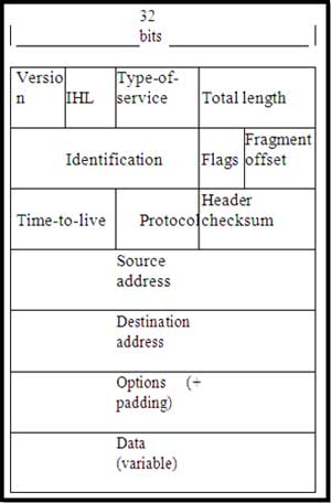
Figure: Fourteen fields comprise an IP packet.
The following discussion describes the IP packet fields illustrated in Figure:
Version: Indicates the version of IP currently used.
IP Header Length (IHL): Indicates the datagram header length in 32-bit words.
Type-of-Service: Specifies how an upper-layer protocol would like a current datagram to be handled, and assigns datagrams various levels of importance.
Total Length: Specifies the length, in bytes, of the entire IP packet, including the data and header.
Identification: Contains an integer that identifies the current datagram. This field is used to help piece together datagram fragments.
Flags: Consists of a 3-bit field of which the two low-order (least-significant) bits control fragmentation. The low-order bit specifies whether the packet can be fragmented. The middle bit specifies whether the packet is the last fragment in a series of fragmented packets. The third or high-order bit is not used.
Fragment Offset: Indicates the position of the fragment’s data relative to the beginning of the data in the original datagram, which allows the destination IP process to properly reconstruct the original datagram.
Time-to-Live: Maintains a counter that gradually decrements down to zero, at which point the datagram is discarded. This keeps packets from looping endlessly.
Protocol: Indicates which upper-layer protocol receives incoming packets after IP processing is complete.
Header Checksum: Helps ensure IP header integrity.
Source Address: Specifies the sending node.
Destination Address: Specifies the receiving node.
Options: Allows IP to support various options, such as security.
Data: contains upper layer information
IP ADDRESSING
As with any other network-layer protocol, the IP addressing scheme is integral to the process of routing IP datagrams through an internetwork. Each IP address has specific components and follows a basic format. These IP addresses can be subdivided and used to create addresses for sub networks, as discussed in detail later in this chapter.
Each host on a TCP/IP network is assigned a unique 32-bit logical address that is divided into two main parts: the network number and the host number. The network number identifies a network and must be assigned by the Internet Network Information Center (InterNIC), if the network is to be part of the Internet. An Internet Service Provider (ISP) can obtain blocks of network addresses from the InterNIC and can itself assign address space as necessary. The host number identifies a host on a network and is assigned by the local network administrator.
IP Address Format
The 32-bit IP address is grouped eight bits at a time, separated by dots, and represented in decimal format (known as dotted decimal notation). Each bit in the octet has a binary weight (128, 64, 32, 16, 8, 4, 2, 1). The minimum value for an octet is 0, and the maximum value for an octet is 255. Figure illustrates the basic format of an IP address.
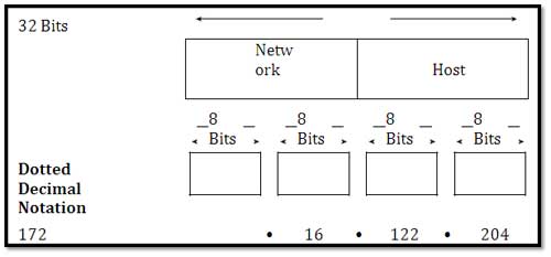
Figure: An IP address consists of 32 bits, grouped into four octets.
IP Address Classes
IP addressing supports five different address classes: A, B,C, D, and E. Only classes A, B, and C are available for commercial use. The left-most (high-order) bits indicate the network class. Table below provides reference information about the five IP address classes.
| IP Address Class | Format | Purpose | High-Order Bit(s) | Address Range | No. Bits Network/ Host | Max. Hosts |
| A | N.H.H.H1 | Few large | 0 | 1.0.0.0 to 126.0.0.0 | 7/24 | 16,777, 2142 |
| organizations | (224 – 2) | |||||
| B | N.N.H.H | Medium-size | 1, 0 | 128.1.0.0 to | 14/16 | 65, 543 (216 – |
| organizations | 191.254.0.0 | 2) | ||||
| C | N.N.N.H | Relatively small | 1, 1, 0 | 192.0.1.0 to | 22/8 | 245 (28 – 2) |
| organizations | 223.255.254.0 | |||||
| D | N/A | Multicast groups | 1, 1, 1, 0 | 224.0.0.0 to | N/A (not for | N/A |
| (RFC 1112) | 239.255.255.255 | commercial use) | ||||
| E | N/A | Experimental | 1, 1, 1, 1 | 240.0.0.0 to | N/A | N/A |
| 254.255.255.255 |
- N = Network number, H = Host number.
- One address is reserved for the broadcast address, and one address is reserved for the network.
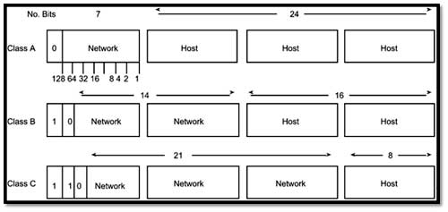
Figure: IP address formats A, B, and C are available for commercial use.
The class of address can be determined easily by examining the first octet of the address and mapping that value to a class range in the following table. In an IP address of 172.31.1.2, for example, the first octet is 172. Because 172 falls between 128 and 191, 172.31.1.2 is a Class B address. Figure summarizes the range of possible values for the first octet of each address class.
| Address Class | First Octet in Decimal | High-Order Bits |
| Class A | 1 - 126 | 0 |
| Class B | 128 - 191 | 10 |
| Class C | 192 - 223 | 110 |
| Class D | 224 - 239 | 1110 |
| Class E | 240 - 254 | 1111 |
IP Subnet Addressing
IP networks can be divided into smaller networks called subnetworks (or subnets). Subnetting provides the network administrator with several benefits, including extra flexibility, more efficient use of network addresses, and the capability to contain broadcast traffic (a broadcast will not cross a router).
Subnets are under local administration. As such, the outside world sees an organization as a single network and has no detailed knowledge of the organization’s internal structure.
A given network address can be broken up into many subnetworks. For example, 172.16.1.0, 172.16.2.0, 172.16.3.0, and 172.16.4.0 are all subnets within network 171.16.0.0. (All 0s in the host portion of an address specifies the entire network.)
IP Subnet Mask
A subnet address is created by “borrowing” bits from the host field and designating them as the subnet field. The number of borrowed bits varies and is specified by the subnet mask. Figure shows how bits are borrowed from the host address field to create the subnet address field.
Class B Address: Before Subnetting
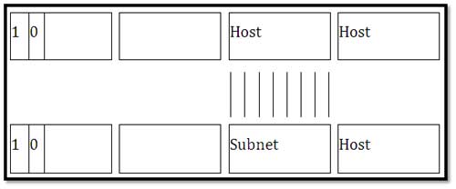
Figure: Bits are borrowed from the host address field to create the subnet address field.
Class B Address: After Subnetting
Subnet masks use the same format and representation technique as IP addresses. The subnet mask, however, has binary 1s in all bits specifying the network and subnetwork fields, and binary 0s in all bits specifying the host field. Figure 30-7 illustrates a sample subnet mask.
|
| Network | Network | Subnet | Host |
| Binary Representation | 11111111 | 11111111 | 11111111 | 00000000 |
| Dotted decimal Representation | 255 | 255 | 255 | 0 |
Subnet mask bits should come from the high-order (left-most) bits of the host field, as below figure illustrates. Details of Class B and C subnet mask types follow. Class A addresses are not discussed in this chapter because they generally are subnetted on an 8-bit boundary.
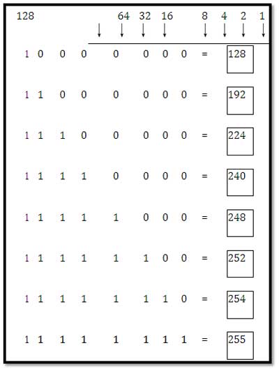
Figure: Subnet mask bits come from the high-order bits of the host field.
Various types of subnet masks exist for Class B and C subnets.
The default subnet mask for a Class B address that has no subnetting is 255.255.0.0, while the subnet mask for a Class B address 171.16.0.0 that specifies eight bits of subnetting is 255.255.255.0. The reason for this is that eight bits of subnetting or 28 – 2 (1 for the network address and 1 for the broadcast address) = 254 subnets possible, with 28 – 2 = 254 hosts per subnet.
The subnet mask for a Class C address 192.168.2.0 specifies five bits of subnetting is 255.255.255.248. With five bits available for subnetting, 25 – 2 = 30 subnets possible, with 23 – 2 = 6 hosts per subnet.
The reference charts shown in tables below can be used when planning Class B and C networks to determine the required number of subnets and hosts, and the appropriate subnet mask.
Table: Class B Subnetting Reference Chart
| Number of Bits | Subnet Mask | Number of Subnets | Number of Hosts |
| 2 | 255.255.192.0 | 2 | 16382 |
| 3 | 255.255.224.0 | 6 | 8190 |
| 4 | 255.255.240.0 | 14 | 4094 |
| 5 | 255.255.248.0 | 30 | 2046 |
| 6 | 255.255.252.0 | 62 | 1022 |
| 7 | 255.255.254.0 | 126 | 510 |
| 8 | 255.255.255.0 | 254 | 254 |
| 9 | 255.255.255.128 | 510 | 126 |
| 10 | 255.255.255.192 | 1022 | 62 |
| 11 | 255.255.255.224 | 2046 | 30 |
| 12 | 255.255.255.240 | 4094 | 14 |
| Number of Bits | Subnet Mask | Number of Subnets | Number of Hosts |
| 13 | 255.255.255.248 | 8190 | 6 |
| 14 | 255.255.255.252 | 16382 | 2 |
| Table | Class C Subnetting Reference Chart | ||
| Number of Bits | Subnet Mask | Number of Subnets | Number of Hosts |
| 2 | 255.255.255.192 | 2 | 62 |
| 3 | 255.255.255.224 | 6 | 30 |
| 4 | 255.255.255.240 | 14 | 14 |
| 5 | 255.255.255.248 | 30 | 6 |
| 6 | 255.255.255.252 | 62 | 2 |