Transaction Flow Testing

Introduction:
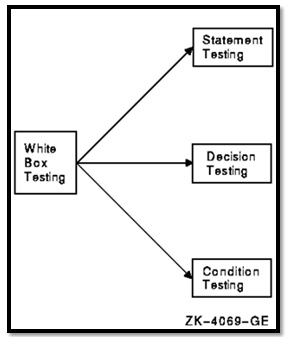
White box testing is a testing technique that examines the program structure and derives test data from the program logic/code. The other names of glass box testing are clear box testing, open box testing, logic driven testing or path driven testing or structural testing.

White box testing is also known as structured based. This structured based testing techniques which are also dynamic rather than static use the internal structure of the software to derive the test cases they are commonly called white box or glass box techniques. Implying you can see into the system since they required knowledge of how the software is implemented that is how it works, for example, a structural technique may be concerned with the excising loops in the software.

White Box Testing Techniques:

• Statement Coverage - This technique is aimed at exercising all programming statements with minimal tests.
• Branch Coverage - This technique is running a series of tests to ensure that all branches are tested at least once.
• Path Coverage - This technique corresponds to testing all possible paths which mean that each statement and branch is covered.

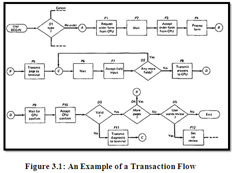
A transaction is a unit of work seen from a system user's point of view. A transaction consists of a sequence of operations, some of which are performed by a system, persons or devices that are outside of the system. Transaction begins with Birth that is they are created as a result of some external act. At the conclusion of the transaction's processing, the transaction is no longer in the system.

Example of a transaction: A transaction for an online information retrieval system might consist of the following steps or tasks:

• Accept input (tentative birth)
• Validate input (birth)
• Transmit acknowledgment to requester
• Do input processing
• Search file
• Request directions from user
• Accept input
• Validate input
• Process request
• Update file
• Transmit output
• Record transaction in log and clean up (death)

TRANSACTION FLOW GRAPHS:

• Transaction flows are introduced as a representation of a system's processing.
• The methods that were applied to control flow graphs are then used for functional testing.
• The transaction flow graph is to create a behavioral model of the program that leads to functional testing.
• The transaction flowgraph is a model of the structure of the system's behavior (functionality).
• An example of a Transaction Flow is as follows:

USAGE:

• Transaction flows are indispensable for specifying requirements of complicated systems, especially online systems.
• A big system such as an air traffic control or airline reservation system has not hundreds, but thousands of different transaction flows.
• The flows are represented by relatively simple flow graphs, many of which have a single straight-through path.
• Loops are infrequent compared to control flow graphs.
• The most common loop is used to request a retry after user input errors. An ATM system, for example, allows the user to try, saying three times, and will take the card away the fourth time.

COMPLICATIONS:

• In simple cases, the transactions have a unique identity from the time they're created to the time they're completed.
• In many systems, the transactions can give birth to others, and transactions can also merge.

Births
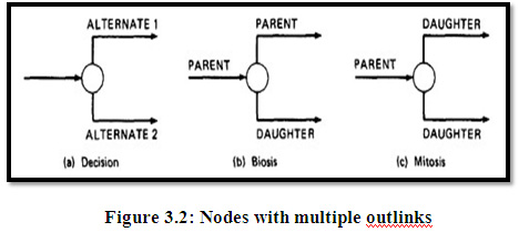
There are three different possible interpretations of the decision symbol or nodes with two or more out links. It can be a Decision, Biosis or a Mitosis.

Decision
Here the transaction will take one alternative or the other alternative but not both. (See Figure 3.2 (a))

Biosis
Here the incoming transaction gives birth to a new transaction, and both transactions that continue on their separate paths and the parent retains its identity. (See Figure 3.2 (b))

Mitosis
Here the parent transaction is destroyed and two new transactions are created.(See Figure 3.2 (c))

Mergers
Transaction flow junction points are potentially as troublesome as transaction flow splits. There are three types of junctions: (1) Ordinary Junction (2) Absorption (3) Conjugation

Ordinary Junction: An ordinary junction which is similar to the junction in a control flow graph. A transaction can arrive either on one link or the other. (See Figure 3.3 (a))

Absorption: In absorption case, the predator transaction absorbs prey transaction. The prey was gone but the predator retains its identity. (See Figure 3.3 (b))

Conjugation: In conjugation case, the two parent transactions merge to form a new daughter. In keeping with the biological flavor, this case is called as conjugation.

Transaction Flow Testing Techniques:
Get The Transactions Flows:

• Complicated systems that process a lot of different, complicated transactions should have explicit representations of the transactions flows, or the equivalent.
• Transaction flows are like control flow graphs, and consequently we should expect to have them in increasing levels of detail.
• The system's design documentation should contain an overview section that details the main transaction flows.
• Detailed transaction flows are a mandatory prerequisite to the rational design of a system's functional test.

Inspections, Reviews and Walkthroughs:

• Transaction flows are natural agenda for system reviews or inspections.
• In conducting the walkthroughs, you should:
• Discuss enough transaction types to account for 98%-99% of the transaction the system is expected to process.
• Discuss paths through flows in functional rather than technical terms.
• Ask the designers to relate every flow to the specification and to show how that transaction, directly or indirectly, follows from the requirements.
• Make transaction flow testing the cornerstone of system functional testing just as path testing is the cornerstone of unit testing.
• Select additional flow paths for loops, extreme values, and domain boundaries.
• Design more test cases to validate all births and deaths.
• Publish and distribute the selected test paths through the transaction flows as early as possible so that they will exert the maximum beneficial effect on the project.

Path Selection:

• Select a set of covering paths (c1+c2) using the analogous criteria that were used for structural path testing.
• Select a covering set of paths based on functionally sensible transactions, as you would for control flow graphs.
• Try to find the most tortuous, longest, strangest path from the entry to the exit of the transaction flow.

Path Sensitization:

• Add your content...Most of the normal paths are very easy to sensitize-80% - 95% transaction flow coverage (c1+c2) is usually easy to achieve.
• The remaining small percentage is often very difficult.
• Sensitization is the act of defining the transaction. If there are sensitization problems on the easy paths, then bet on either a bug in transaction flows or a design bug.

Path Instrumentation:

• Instrumentation plays a bigger role in transaction flow testing than in unit path testing.
• The information of the path taken for a given transaction must be kept with that transaction and can be recorded by a central transaction dispatcher or by the individual processing modules.
• In some systems, such traces are provided by the operating systems or a running log.

Data Flow Testing:
Data flow testing is the name given to a family of test strategies based on selecting paths through the program's control flow in order to explore sequences of events related to the status of data objects. For example, pick enough paths to assure that every data object has been initialized prior to use or that all defined objects have been used for something.

Motivation: It is our belief that, just as one would not feel confident about a program without executing every statement in it as part of some test, one should not feel confident about a program without having seen the effect of using the value produced by each and every computation.

Data Flow Machines:
There are two types of data flow machines with different architectures. (1) Von Neumann machines (2) Multi-instruction, multi-data machines (MIMD).

Von Neumann Machine Architecture:

• Most computers today are Von-Neumann machines.
• This architecture features interchangeable storage of instructions and data in the same memory units.
• The Von Neumann machine Architecture executes one instruction at a time in the following, micro instruction sequence:
• Fetch instruction from memory
• Interpret instruction
• Fetch operands

1. Process or Execute
2. Store result
3. Increment program counter
4. GOTO 1

Multi-instruction, Multi-data machines (MIMD) Architecture:

• These machines can fetch several instructions and objects in parallel.
• They can also do arithmetic and logical operations simultaneously on different data objects.
• The decision of how to sequence them depends on the compiler.

Bug Assumption:

• The bug assumption for data-flow testing strategies is that control flow is generally correct and that something has gone wrong with the software so that data objects are not available when they should be, or silly things are being done to data objects.
• Also, if there is a control-flow problem, we expect it to have symptoms that can be detected by data-flow analysis.
• Although we'll be doing data-flow testing, we won't be using data flow graphs as such. Rather, we'll use an ordinary control flow graph annotated to show what happens to the data objects of interest at the moment.

Data Flow Graphs:

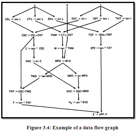
• The data flow graph is a graph consisting of nodes and directed links.
  
• We will use a control graph to show what happens to data objects of interest at that moment.
• Our objective is to expose deviations between the data flows we have and the data flows we want.

Data Object State and Usage:

• Data Objects can be created, killed and used.
• They can be used in two distinct ways: (1) In a Calculation (2) As a part of a Control Flow Predicate.
• The following symbols denote these possibilities:
• Defined: d - defined, created, initialized etc
• Killed or undefined: k - killed, undefined, released etc

Usage: u - used for something (c - used in Calculations, p - used in a predicate)
Defined (d):

• An object is defined explicitly when it appears in a data declaration.
• Or implicitly when it appears on the left hand side of the assignment.
• It is also to be used to mean that a file has been opened.
• A dynamically allocated object has been allocated.
• Something is pushed on to the stack.
• A record written.

Killed or Undefined (k):

• An object is killed on undefined when it is released or otherwise made unavailable.
• When its contents are no longer known with certitude (with absolute certainty / perfectness).
• Release of dynamically allocated objects back to the availability pool.
• Return of records.
• The old top of the stack after it is popped.
• An assignment statement can kill and redefine immediately. For example, if A had been previously defined and we do a new assignment such as A : = 17, we have killed A's previous value and redefined A

Usage (u):

• A variable is used for computation (c) when it appears on the right hand side of an assignment statement.
• A file record is read or written.
• It is used in a Predicate (p) when it appears directly in a predicate.

Data Flow Anomalies:

• An anomaly is denoted by a two-character sequence of actions.
• For example, ku means that the object is killed and then used, where as dd means that the object is defined twice without an intervening usage.
• What is an anomaly is depend on the application.
• There are nine possible two-letter combinations for d, k and u. some are bugs, some are suspicious, and some are okay.
  1. dd :- probably harmless but suspicious. Why define the object twice without an intervening usage?
  2. dk :- probably a bug. Why define the object without using it?
  3. du :- the normal case. The object is defined and then used.
  4. kd :- normal situation. An object is killed and then redefined.
  5. kk :- harmless but probably buggy. Did you want to be sure it was really killed?
  6. ku :- a bug. the object doesnot exist.
  7. ud :- usually not a bug because the language permits reassignment at almost any time.
  8. uk :- normal situation.
  9. uu :- normal situation.
• In addition to the two letter situations, there are six single letter situations.
• We will use a leading dash to mean that nothing of interest (d,k,u) occurs prior to the action noted along the entry-exit path of interest.
• A trailing dash to mean that nothing happens after the point of interest to the exit.
• They possible anomalies are:
  1. -k :- possibly anomalous because from the entrance to this point on the path, the variable had not been defined. We are killing a variable that does not exist.
  2. -d :- okay. This is just the first definition along this path.
  3. -u :- possibly anomalous. Not anomalous if the variable is global and has been previously defined.
  4. k- :- not anomalous. The last thing done on this path was to kill the variable.
  5. d- :- possibly anomalous. The variable was defined and not used on this path. But this could be a global definition.
  6. u- :- not anomalous. The variable was used but not killed on this path. Although this sequence is not anomalous, it signals a frequent kind of bug. If d and k mean dynamic storage allocation and return respectively, this could be an instance in which a dynamically allocated object was not returned to the pool after use.

Data Flow Anomaly State Graph:

• Data flow anomaly model prescribes that an object can be in one of four distinct states:
  • K :- undefined, previously killed, does not exist
  • D :- defined but not yet used for anything
  • U :- has been used for computation or in predicate
  • A :- anomalous
• These capital letters (K, D, U, A) denote the state of the variable and should not be confused with the program action, denoted by lower case letters.
• Unforgiving Data - Flow Anomaly Flow Graph: Unforgiving model, in which once a variable becomes anomalous it can never return to a state of grace.

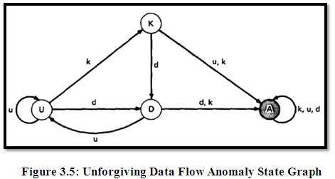
Assume that the variable starts in the K state - that is, it has not been defined or does not exist. If an attempt is made to use it or to kill it (e.g., say that we're talking about opening, closing, and using files and that 'killing' means closing), the object's state becomes anomalous (state A) and, once it is anomalous, no action can return the variable to a working state. If it is defined (d), it goes into the D, or defined but not yet used, state. If it has been defined (D) and redefined (d) or killed without use (k), it becomes anomalous, while usage (u) brings it to the U state. If in U, redefinition (d) brings it to D, u keeps it in U, and k kills it.

Forgiving Data - Flow Anomaly Flow Graph
Forgiving model is an alternate model where redemption (recover) from the anomalous state is possible.

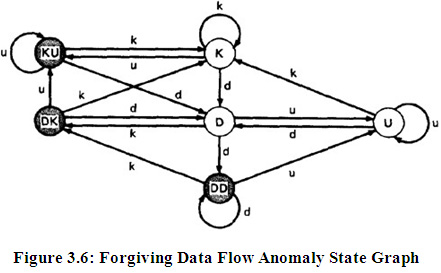
This graph has three normal and three anomalous states and he considers the kk sequence not to be anomalous. The difference between this state graph and Figure 3.5 is that redemption is possible. A proper action from any of the three anomalous states returns the variable to a useful working state.
The point of showing you this alternative anomaly state graph is to demonstrate that the specifics of an anomaly depends on such things as language, application, context, or even your frame of mind. In principle, you must create a new definition of data flow anomaly (e.g., a new state graph) in each situation. You must at least verify that the anomaly definition behind the theory or imbedded in a data flow anomaly test tool is appropriate to your situation.

Static Vs Dynamic Anomaly Detection:

• Static analysis is analysis done on source code without actually executing it. For example: source code syntax error detection is the static analysis result.
• Dynamic analysis is done on the fly as the program is being executed and is based on intermediate values that result from the program's execution. For example: a division by zero warning is the dynamic result.
• If a problem, such as a data flow anomaly, can be detected by static analysis methods, then it doesn’t belong in testing - it belongs in the language processor.
• There is actually a lot more static analysis for data flow analysis for data flow anomalies going on in current language processors.
• For example, language processors which force variable declarations can detect (-u) and (ku) anomalies.
• But still there are many things for which current notions of static analysis are INADEQUATE.

Data Flow Model:

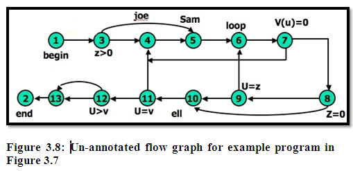
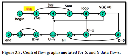
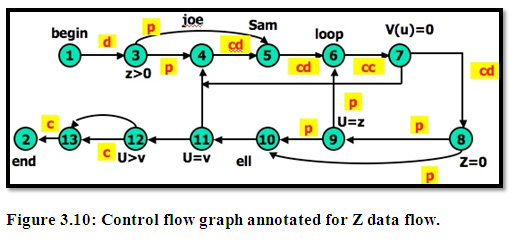
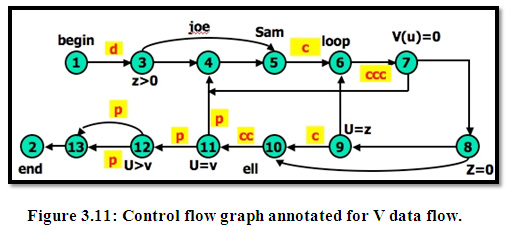
• The data flow model is based on the program's control flow graph - Don't confuse that with the program's data flow graph.
• Here we annotate each link with symbols (for example, d, k, u, c, p) or sequences of symbols (for example, dd, du, ddd) that denote the sequence of data operations on that link with respect to the variable of interest. Such annotations are called link weights.
• The control flow graph structure is same for every variable: it is the weights that change.

Example:

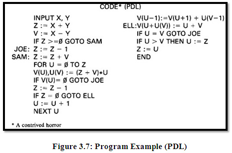
Data flow testing is a family of test strategies based on selecting paths through the program's control flow in order to explore sequences of events related to the status of variables or data objects. Dataflow Testing focuses on the points at which variables receive values and the points at which these values are used.

Published date : 14 Jul 2015 04:59PM